Inherent variability in energy testing of CI pipelines
- by Dan Mateas

As we’ve been testing the energy use of various CI pipelines using Eco-CI, one thing we’ve noticed is that there is a large amount of variability in the results. Pipeline runs that we would expect to be more or less the same (same commit hash, running a few days in a row on the same cpu) can have wildly different results:

Energy cost of a test pipeline on Github. y-axis is in mJ. Up to 30% difference.

Some amount of this is to be expected - using shared runners you don’t have full control of your machine and don’t really know what else could be running, and not all pipelines run in a fixed amount of steps. Still, this variability was higher than we expected, so we asked ourselves: what’s the inherent variability that we must expect when energy testing ci pipelines? Can we find any explanation for this variability, and how to account for it when measuring CI pipelines? That’s what we are exploring today.

What do we want to find out?

Research question
How is the energy variance in hosted pipelines (Github/Gitlab) and can we use it for energy optimizations?

Setup

First, we made a simple pipeline that should run in a relatively consistent amount of time/steps. All the pipeline does is install and runs sysbench:

 - name: Install sysbench
        run: |
          sudo time apt install sysbench -y
                    
      # Runs a single command using the runners shell
      - name: Running sysbench
        run: |
          time sysbench --cpu-max-prime=25000 --threads=1 --time=0 --test=cpu run --events=20000 --rate=0          


We added Eco-CI into this, and measured two distinct steps: first the installation process, and then running the sysbench command. We ran this many times over a few days and looked at the energy and time used, as well as the average cpu utilization for each step. We then calculated the mean and standard deviance for these values.

We also keep track which cpu each run is being done on. As a refresher, the ML model that Eco-CI is based on identifies CPU model and utilization as the biggest contributing factors towards the energy use of servers. This means that comparing runs across different CPU’s is unfair - one cpu model might inherently cost more energy for your run. While very interesting information in its own right, for the purposes of calculating variability we can only calculate the mean and standard deviance for each cpu seperately.

We also ran this pipeline on Gitlab, and gathered the same data. Gitlab hosted runners only have one cpu, so that simplifies things a bit.

So after gathering the data from both Github and Gitlab and calculating the statistics, here’s the results we found, by platform/CPU:

Platform/CPU Step Energy Mean Energy Std.Dev (Value / %) Time Mean Time Std. Dev (value/%) Avg. Cpu. Utilization Count
Github / 8171M Install Step 60.4 J 36.4 J / 60% 18s 8s / 43% 35% 75
Run Step 380 J 16.2 J / 4% 86s 4s / 4% 48% 75
Full Pipeline 440.9 J 42.6 J / 10% 104s 9s / 9% 42% 75
Github / 8272CL Install Step 53.1 J 55.6 J / 105% 16s 12s / 75% 32% 81
Run Step 327.7 J 1.2 J / 0% 74s 1s / 1% 48% 81
Full Pipeline 380.8 J 55.8 J / 15% 90s 12s / 13% 40% 81
Github / E5-2673v4 Install Step 73.7 J 55.5 J / 75% 19s 11s / 58% 35% 55
Run Step 404.1 J 37.6 J / 9% 85s 8s / 9% 48% 55
Full Pipeline 477.9 J 75.8 J / 16% 104s 15s / 15% 42% 55
Github / E5-2673v3 Install Step 69.9 J 3.8 J / 6% 13s 0s / 4% 32% 10
Run Step 594.8 J 24.6 J / 4% 85s 3s / 4% 48% 10
Full Pipeline 664.8 J 26.1 J / 4% 98s 4s / 4% 40% 10
Github / 8370C Install Step 48.4 J 32.3 J / 67% 16s 8s / 48% 32% 52
Run Step 146.9 J 0.4 J / 0% 39s 0s / 1% 45% 52
Full Pipeline 195 J 32 J / 16% 56s 8s / 14% 38% 52
Gitlab / EPYC_7B12 Install Step 10.6 J 9.7 J / 92% 5s 3s / 51% 53% 196
Run Step 54.2 J 3.8 J / 7% 20s 0s / 2% 57% 196
Full Pipeline 64.8 J 6.4 J / 10% 25s 3s / 10% 55% 196
Analysis

There’s a lot of numbers up there, but let’s see if we can summarize some conclusions from this.

Looking at the entire pipeline as one overall energy measurement, we can see that the variability (standard deviation % of energy consumed) is large and spans a wide margin: anywhere from 4% - 16%. However when we break it down to installation / running steps, we notice a drastic split - the installation step consistently has a much wider variability (6 - 105(!!)%), while the run sysbench step has a much more narrow variability (0-9%).

Looking through the job logs for the installation step it becomes apparent that network traffic speeds accounts for quite a bit of this variability. Jobs whose package downloads were slower (even if they’re the same packages) took an expectedly longer amount of time. This explains the time variability, and corresponding energy variability we see.

This highlights the importance of breaking down your pipeline when making energy estimations for the purposes of optimizing gains. You generally do not have much control over network speeds, though you can try to minimize network traffic. Fortunately, if we look at the energy breakdown, we can see that both the energy consumed and cpu utilization were lower across the board for the install steps. So while these sections have a large variability, they also account for a minority of the energy cost.

Looking at just the running steps, which accounts for the majority of the energy cost, we notice two things. First - the energy standard deviation % and time standard deviation % are almost identical in most cases (Gitlab’s EPYC_7B12 being the odd one out, though the two numbers are still comparable). This means that we have a pattern here that the longer a job takes, we have a proportionally larger energy cost - which is what we would expect.

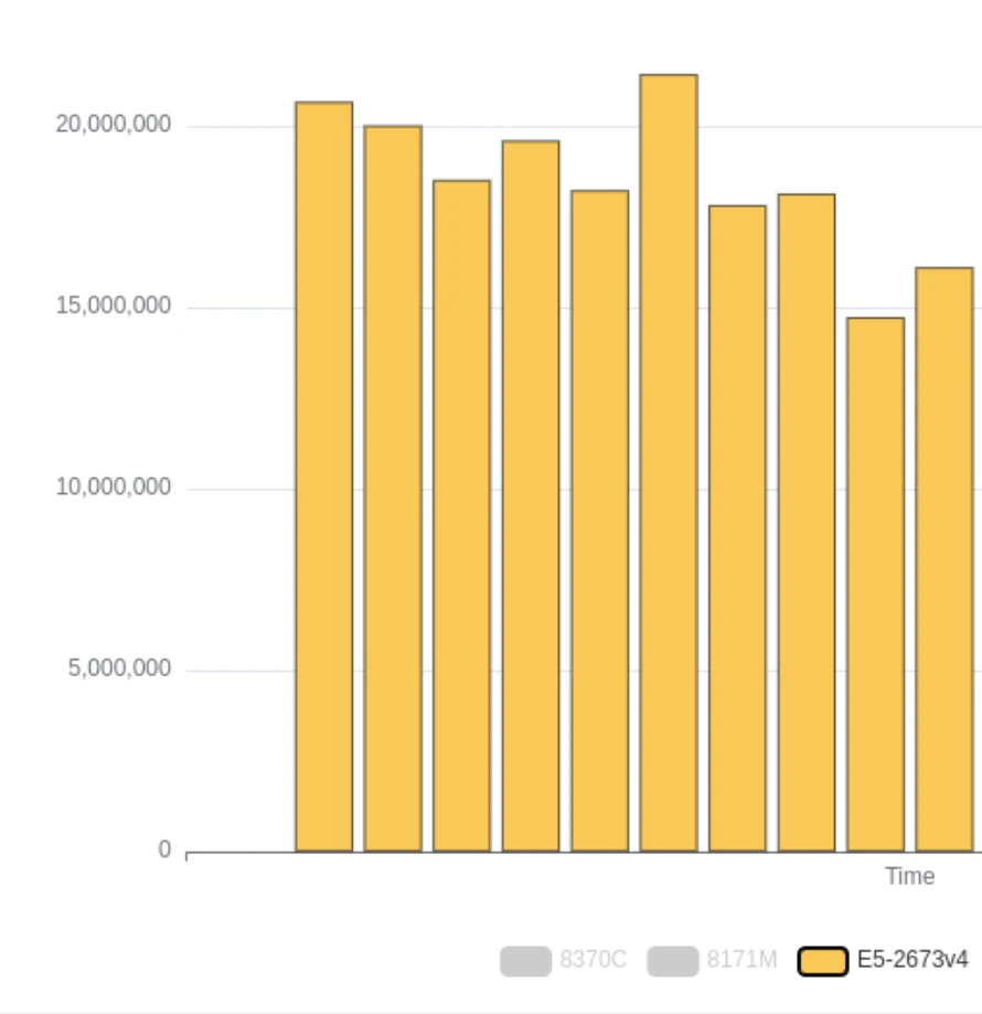
We also notice that the baseline standard deviation we are calculating here seems to be very CPU dependent. Certain CPU’s such as the 8370C and 8272CL seem to perform more consistently than others. Their standard deviation is very low - 0-1%.

Running these tests a few times over a few weeks, these patterns regarding CPU still held.

Conclusions

So what did we gather from this analysis, and how can we integrate this knowledge in our quest for energy optimizations? Generally speaking, when we analyze our pipelines over a period of time, we want to know if a change we’ve made has increased or decreased our energy usage. Big changes (such as ones that cause our pipelines to run twice as long) will have obvious impacts. However, if we want to optimize our pipelines without changing inherent functionality, then examinging the variability becomes important. We want to know if our small change made a real difference, and if the inherent variability is larger than the change’s impact, then it becomes indistinguisable from noise.

With that in mind, what we measure in our pipelines is important. Any steps that include have network traffic, will have too high of an inherent variability for us to make a meaningful analysis. These steps have variability of upwards to 40-100%, so unless the change is drastic enough to consistently cause your pipeline use double the energy of previous runs, any practical changes will be lost amongst the noise.

When we strip down to steps that are just local machine calculations , then we see the variability is much more managable. It is still very cpu dependant however. Here are the results summarized:

Platform/CPU Energy Variability Time Variability
Github / 8272CL 0% 1%
Github / 8370C 0% 1%
Github / 8171M 4% 4%
Github / E5-2673v3 4% 4%
Gitlab / EPYC_7B12 7% 2%
Github / E5-2673v4 9% 9%

So if you want to measure the impact of optimziations on your pipelines, you have to pay attention to which CPU your workflow is running on. Github runners on 8370C and 8272CL machines are the best to examine to accurately see what impact your pipeline changes have. Any optimization should be accurately reflected on thse machines. For any changes that cause a 4% or less energy use impact, examining pipeline runs on other machines may lead to inaccurate conclusions.

Obviously this is only an observed and snapshotted result, so this might change in the future unannounced. We have scheduled to revisit this test in a couple of months to see if any changes happended.

In the meantime we are also very happy to link out to any reproductions of this test that can falsify if you get similar results to ours.